Studies of Performance on a Mathematics Entrance Examination for the University of Macau
Dr.David Laffie and Zhao Ping,Peggy(Faculty of Social Sciences and Humanities,University of Macau)
澳門大學數學入學考試成績分析
本文用統計方法對1990年澳門大學數學入學考試成績進行了詳盡的分析。它介紹了考生成績的統計分配情況,並對入學考試成績是否能準確地預測大學一年級數學成績的問題進行了分析。利用考生所提供的個人資料,本文還闡述了入學考試成績與考的各種社會因素間的相關關係。分析結果表明,入學考試成績與大學一年級數學成績基不相關。男考生與女考生的成績沒有明顯差別。入學考試成績與年龄呈負相關。年齡越小,成績越高。某些中學的考生成績高於整體水平,而另一些學校的考生成績則低於整體水平。中國考生的成績顯著高於其他考生,而香港考生成績則相對較低。雖然入學考試成績與監護人及其職業間的關係不如其他因素明顯,本文對些也進行了討論。
INTRODUCTION
In May and June, 1990, the first annual Entrance Examinations for admission to the University of Macau were offered to prospective first year students. The Mathematics B examination was offered in two sittings spaced about a month apart. This examination was intended for those applicants who wished to be considered for admission to the Faculty of Business Administration, the Faculty of Social Science or the Faculty of Education. The two examination papers given at these two sittings were different although they were similar in content since they were written from the same examination syllabus by the same authors. One of us (DL) was one of two authors of the examination papers. Both of the present authors were among those responsible for teaching the first year mathematics in the Faculty of Business Administration to the students who entered. This situation presented us with an opportunity to examine the performance of the students we were teaching on Entrance Examinations and to trace their progress through the first year of mathematics courses. Some interesting results have emerged from the study and we hope that they will provide the stimulus needed to collect further data on future applicants and possibly to generate other studies in this area.
Students who took the examinations fell into three groups:
Group Ⅰ: Those who took the examination at the first sitting.
Group Ⅱ: Those who took the examination only at the second sitting.
Group Ⅲ: Those who took the examination twice. (Members of Group Ⅲ are also cou-nted in Group Ⅰ.)
From these three groups we constructed a fourth group:
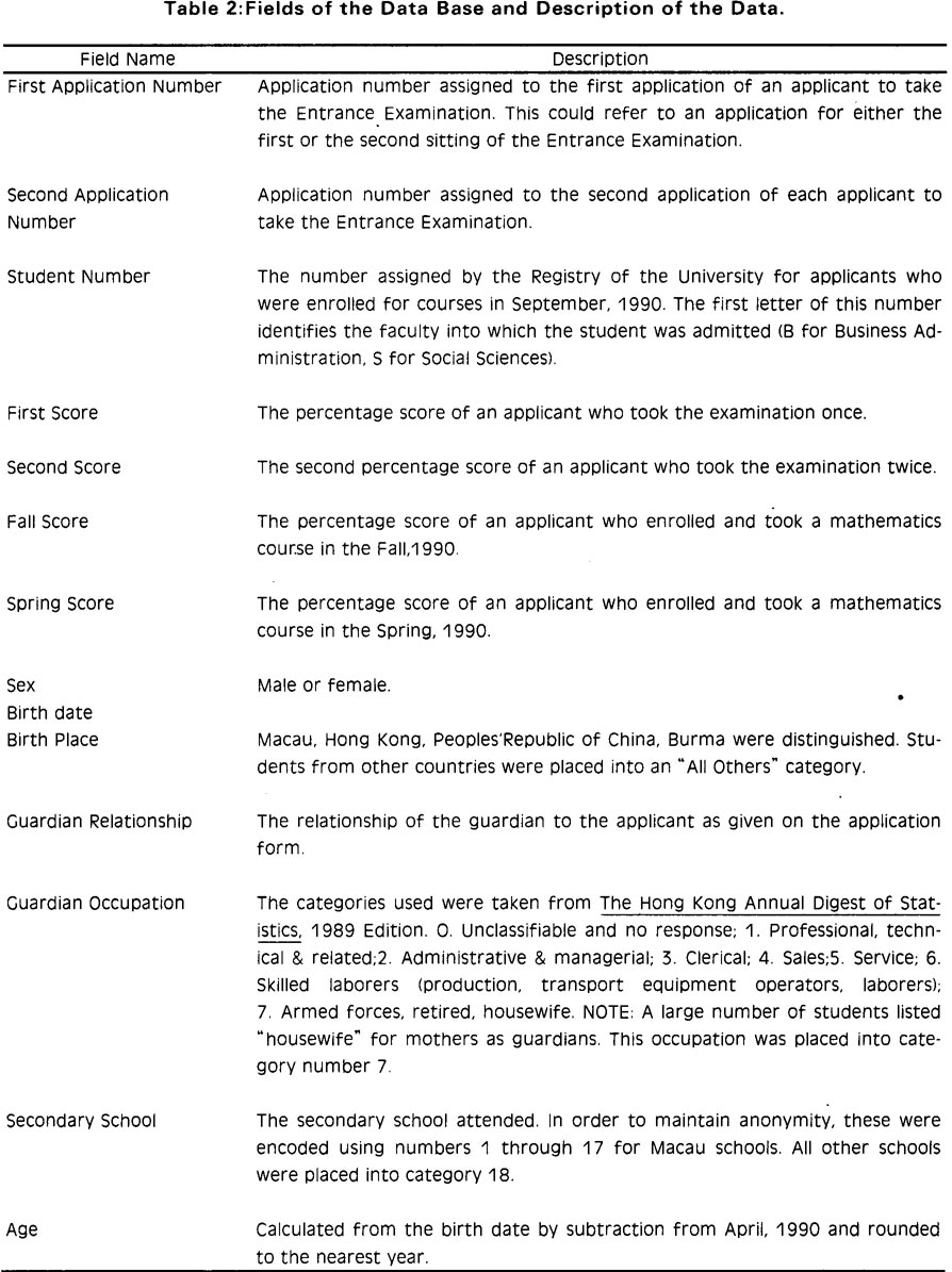
Group Ⅳ: First scores of all those who took the examination. This group is the sum of Group Ⅰ and Group Ⅱ.
The sizes of the four groups are shown in Table 1.
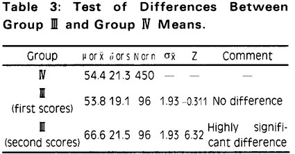
In addition to the scores for the two Entrance Examinations, we obtained the following data from application forms which the applicants filled out: sex, birth date, place of birth, secondary school, relationship of the legal guardian to the applicant, and occupation of the guardian. Using the application numbers, we were able to locate applicants who enrolled in September, 1990 in either the Faculty of Business Administration or the Faculty of Social Sciences. (The Faculty of Education did not offer a mathematics course to their first year students.) Thus we added to the above data: student number, score in the Fall 1990 mathematics course, and score in the Spring, 1991 mathematics course. The student number allowed us to separate the Social Sciences students from Business students when it was necessary to do so.
Using these data, we investigated the following questions: Were groups Ⅰ, Ⅱ,and Ⅳ normally distributed and did they have the same mean and standard deviation? Were applicants who repeated the examination able to increase their scores? What percentage of those who failed on the first try were able to pass on the second try? Were the applicants who repeated (GroupⅢ) in any way distinguishable from Group Ⅰ ? Were the applicants who took the examination only at the first sitting in any way different from those who took it only at the second sitting? (That is, were Groups Ⅰ and Ⅱdifferent or similar?) Was performance on the Entrance Examination in any way a predictor of performance in the first year mathematics courses? Was there any difference in the performance of male and female applicants, applicants who came from different secondary schools, who were born in different countries, who were different ages, who had different guardians, whose guardians had different occupations?
This paper represents an approach to these questions; not a definitive answer to them. The data are not of sufficiently high quality to allow us to make all statements with a great deal of confidence. Our hope is that data will become available in the future which would allow a more thorough analysis;one which would allow us to get to the root of these and other questions of relevance to the quality of life in Macau.
METHODS
Population and Samples.
In order to define the population for this study, it is instructive to consider how the data was taken. No attempt has been made to take a random sample of the secondary school students of Macau or of any other population. The basis of the sample obtained is actually opportunistic: the data are for all students who applied for admission to the University. This group is in itself a population: the population of graduating Form 6 students who chose to apply for admission. The terminology for population parameters rather than for sample statistics is used in later discussions for this reason.
This group is obviously a sub-population of the total population of graduating Form 6 students, but is not a random sample of that group and therefore the results presented here cannot be used to infer anything about the latter group. It is not the purpose of this paper to provide feedback to the Macau school system regarding the preparation of students for study at the University of Macau. Therefore, readers should be verycautious about interpreting these results. They properly apply only to the students who apply for admission and not to any other population or group of people.
In addition, another factor should be considered in interpreting the results presented here. Many Macau schools offer two tracks of study toward a Form 6 diploma: a technical track and a non--technical track. The Mathematics B examination syllabus was written for the students who had followed the non--technical track. The mathematical level of this track is less demanding than that of the technical track. It is conceivable, however, that even after obtaining a Form 6 diploma in the technical track, a student might elect to apply for admission to a faculty which only requires the non--technical level of competence in mathematics (e.g.Business Administration, Social Sciences, or Education). Such students would have taken the Mathematics B examination. We have no way in this study of assessing the proportion of applicants who fall into this category. Thus is may be that the population of students who took the Mathematics B examination includes students from both tracks.
Original Data and Database Structure
As pointed out in the Introduction, the Entrance Examinations were offered in two sittings. Applicants were allowed to take either examination or both. Therefore some applicants have two scores and others only have one score. Photocopies of the original mark lists containing the application numbers and the percentage marks assigned by the assessors were obtained from the office of the Chief Examiner. Also a list of those applicants who took the examination twice was used to separate them from others who took the Examination only at the second sitting. Letter grades which were assigned to percentage marks were used in one of the analyses reported here. All other analysis was carried out using percentage scores on the examination. A dBASE Ⅲ+ file containing all of the information given by applicants on their application forms, with one exception, was obtained. The exception, the occupation of the guardian as listed by the applicant, was taken directly from the application forms. The actual words used by each applicant to describe the guardian's occupation were recorded and these were classified into one of several standard occupational classes (see Table 2). Finally we obtained the scores assigned by instructors for the first year mathematics courses for each applicant who became a student at the University. All of these data were placed into an EXCEL spreadsheet (Macintosh Ⅱ cx computer). The fields in the data base are listed in Table 2.
Data Analysis
We used standard statistical calculations and methods to arrive at results. Where approp riate, frequency distributions were calculated and these are described in detail in the figure legends.
To determine if the frequency distributions of Groups Ⅰ and Ⅳ were normal distributions, the upper and lower boundaries of each class interval (plus or minus 0.5 as needed to maintain continuity) were converted to z--scores (standard normal variant) using the mean and standard deviation of the population. The proportion of the area under the standard normal curve falling within each class interval was calculated on the basis of the z--scores using a table of areas under the standard normal curve. This proportion times the total number in the population gave the number of applicants whose examination scores were expected to fall within each interval if the population were distributed normally. The expected values were then compared with the actual observations using a x2 test for goodness--of --fit.
To determine if the Entrance Examination Scores were good predictors of the applicants' performance in the first year mathematics course, we plotted the first semester or second semester course scores (percentage values) agairst the first time entrance Examination scores. These scatter plots were fit with a least squares straight line and correlation coefficients were calculated. The correlation coefficients were used to draw conclusions regarding this question.
To determine whether social data were correlated with scores in the Entrance Examinations,we sorted the data base using each field containing data relevant to a given social factor. For example, to determine if applicants from particular secondary schools performed differently from the population, the data base was sorted using the field containing the secondary school code. For each school, the mean ,standard deviation and number of applicants from that school were determined. It is clear that such a sub-group is not a random sample of the population. So, in order to determine if the mean was different from the population mean, a variation of the procedure for measuring differences between means was carried out. It was supposed that a given sub-group, for example, all applicants from school 1, could be compared to that of a hypothetical random sample having the same mean and size taken from the population. Since the population from which these samples were taken (Group Ⅰ) was fairly symmetrical and had only one component (see Results), the means of such random samples would be normally distributed even if the sample size were smaller than 30. Because the population is not strictly normal this assertion will become less valid as the sample size decreases. Thus for very small samples (n=2 to l0)conclusions about differences between their means and the population mean may not be valid. Using the sub-group size (n), the sub-group mean ,the population mean (u= 54.4; Group Ⅳ), and the population standard deviation(σ=21.3; Group Ⅳ), we calculated the standard normal variant, corresponding to the subgroup mean for a normal sampling distribution whose standard deviation would be the standard error of the mean calculated from ó and n. This value is, of course one value that the mean of a random sample of size, n, taken from the population may have. If the fraction of the area under the standard normal curve between ±Z is designated (1-α, then this probability is α Thus for values of Z far from zero the probability that they could be due to random sampling variation alone is α This procedure was carried out for each of the fields containing the following data:sex, birth place, guardian relationship, guardian occupation, secondary school, age.
RESULTS
Distributions and x2 Fits to the Standard Normal Curve.
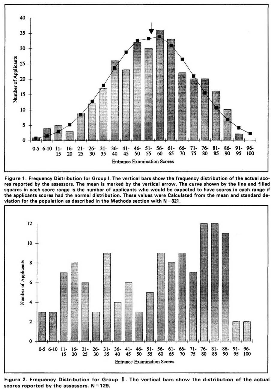
The results from Group I are shown in Figure 1.ln this and succeeding figures the vertical bars show the frequency distribution of the actual scores reported by the assessors. The mean is 54.3. The standard deviation is 18.6. The curve shows a standard normal distribution calculated by the method described in the last section. The x2 analysis showed that the data fit well to a normal curve. Using a null hypothesis that the data fit the normal curve, at the 5% level of significance the critical x2 value is 23.7 (14 degrees of freedom). The value of the test statistic was 16.5. Since 16.5<23.7, we may be confident that the data are normally distributed.
Figure 1.
The results from Group Ⅱ are shown in Figure 2. Here the distribution is distinctly not normal even to the eye. The data appear to fall into two groups which we refer to as Group Ⅱa and Group Ⅱ b. Group Ⅱa is centered approximately on the interval 26-30. Group Ⅱ b is centered approximately on the interval 71-75.
Figure 2.
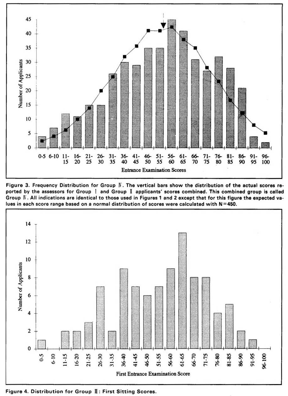
The data for Group Ⅳ are a combination of the data from Groups Ⅰ and Ⅱ. The results for Group Ⅳ are shown in Figure 3. Here we see that the effect of adding the scores of the applicants having a distinctly non-normal distribution (Group Ⅱ) to the scores of the applicants with a normal distribution (Group Ⅰ) is to skew the distribution of all scores towards the high score side of the distribution. The mean is the same as Group Ⅰ (54.4) but the standard deviation is now 21.3. The x2 test indicated that the data are not normally distributed:With 16 degrees of freedom at the 5% level of significance, the critical x2 value is 26.3 whereas the test statistic is 34. Thus at the 5% level of significance the data are not normally distributed. However, the distribution forGroup Ⅳ is fairly symmetrical and has only one componentt, so it is close to a normal distribution. This “nearly normal”aspect of the population will have an affect on conclusions we wish to draw concerning differences of sample means for small random samples (n<30) drawn from this population (see Discussion).
Figure 3.
Results for the Applicants Who Took the Examination Twice:Group Ⅲ
The distribution of first scores of applicants who took the examination twice is shown in Figure 4. The mean and standard deviation were calculated for both the first and the second scores of the applicants. Using the second score values the difference between the mean of the second scores and the mean of the first scores of the entire population (Group Ⅳ) were determined. The difference in these means is highly significant:there is less that 1% chance that this difference could have occurred by random variation. The calculations are shown in Table 3.
Given the equality of the means, standard deviations and distributions of the first scores of Group Ⅲ and the scores from Group Ⅳ (Figure 3) we feel confident in inferring that the applicants who elected to repeat the examination are a random sample of the total group who took it the first time (Group Ⅰ). (Recall that the mean for Group I was 54.3 and the standard deviation was 18.6. See Figure 1.) That is, the ones who repeated are not, as might be expected on a logical basis, primarily the ones who did poorly on the first examination. The mean of the scores on the first examination for this sub-group is not lower than the mean for the whole group.
Figure 4.
In order to further illuminate these results, we determined the mean ,standard deviation and frequency distribution for the differences between scores for each applicant in Group Ⅲ. Those values are mean = +12.8, standard deviation =12.0 (frequency distribution not shown).Thus the applicants who repeated were able to increase their scores by almost 13 percentage points. 10 out of 96 actually lowered their score and 86 out of 96 increased their score by some amount. One person achieved an increase of 61 points.
We also asked the question :what percentage of applicants who failed on the first try were able to pass on the second? The Faculties of Business Administration and Social Sciences used the standard that a grade of C-on the examination would be deemed acceptable for admission. A C-was assigned by the Registry of the University if the applicant received 50 percentage points or higher on the examination. Of the 37 applicants from Group Ⅲ who received less than 50 on the first examination 19 of them received 50 or greater on the second. Thus 51% of the applicants who chose to repeat the examination were able to convert their failing grade to a passing grade.
Predicting Performance in First Year Mathematics Courses
In order to analyze whether results on the Entrance Examination were good predictors of performance in first year mathematics courses, we produced scatter plots from the data base by plotting the Fall course score against the Entrance Examination score for each applicant. We made a second plot using the Spring course scores. Only Business Administration students appeared on the Fall course scores since the Faculty of Social Sciences did not offer a mathema-tics course in Fall. However, in Spring both Faculties gave mathematics courses. Therefore, the students in these faculties were plotted separately and together.
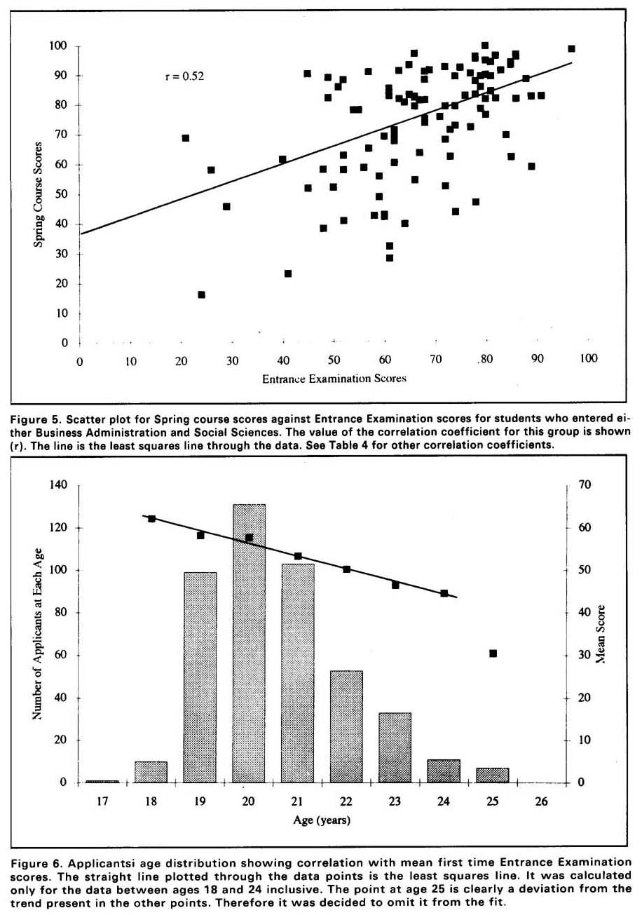
Least squares straight lines were fit to the scatter plots and the correlation coefficients were determined. A high correlation coefficient (close to 1.0),implies that students with a high score on the Entrance Examination will on the average do well in first year mathematics courses. and conversely that an applicant with a low score on the Entrance Examination should do poorly in the first year mathematics courses. The scatter plot for Spring course grades for students from both Business Administration and Social Science is shown in Figure 5. The other three scatter plots look quite similar to this one. The correlation coefficients are listed in Table 4.
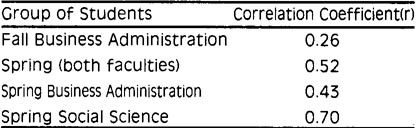
These results indicate that there is essentially no correlation between the score obtained on the Entrance Examinations and the scores obtained by admitted applicants in their first year mathematics courses. The value r=0.7 for students who entered the Faculty of Social Sciences is considerably higher than the others, although it is difficult to explain this result without more data.
Figure 5.
Age of Applicants and Performance on the Entrance Examination.
We sorted the data base using the age field and determined the first score means, standard deviations and frequency for each age within the population. The mean values for each age were plotted on the histogram for the age distribution. These results are shown in Figure 6. the lone applicants aged 17 and 27 were omitted form the plot in Figure 6. It was evident from the plot that the mean examination score when plotted against age approximated a straight line for ages between 18 and 24 (inclusive). A least squares line was calculated for the data of 18-24. This line is also shown in Figure 6. The mean examination scores are strongly correlated with ages: the slope of the line is -3percentage points per year of age between 18 and 24 inclusive. We would need more data in the upper age ranges to determine if the deviation from the trend line at age 25 is significant.
Figure 6.
Possible Relationships Between Social Factors and Performance on the Entrance Examination
We also examined the data for correlations between Entrance Examination scores and the following social factors: sex, place of birth, secondary school, relationship of the legal guardian to the applicant, and occupation of the guardian. In order to carry out these comparisons, we determined the mean and standard deviations for each of subgroup of the population (Group Ⅳ) along with the number in each sub-group. We then compared the mean of each sub-group with the mean of the population using the method of confidence intervals, described in the Methods section of this paper. The results of these comparisons are given in Tables 5-7 and Figures 7-10. Except where noted, all of the Z-scores were calculated for a sampling distribution of the mean with reference to the population mean and standard deviation for Group Ⅳgiven in Table 5.
Sex
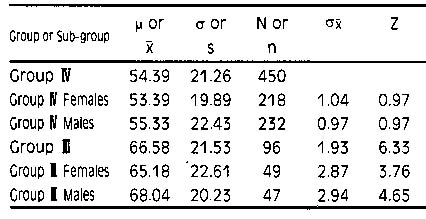
According to the arguments given in the Methods section, if |z|≥1.645, |z|≥1.96, or|z| ≥2.575 then the probabilities that the difference between the observed sub-group mean and the population mean are 0.90, 0.95,or 0.99,respectively. A probability of less than 0.9 is not considered to be statistically meaningful; i.e.we cannot tell the differencebetween the sub-group mean and the mean of a random sample taken from the population. Using this concept, we see that Table 5 indicates that there is no detectable difference between females and males on this Entrance Examination. They have the same means as the population whether they sit once or twice. Also females and males were able to increase their scores by the same amount by repeating the examination (Z--scores comparing the female's and male's second scores to the mean score for the repeated examination are 0.65 (females) and 0. 65(males). Therefore, the females and males who repeated the examination performed equivalently.) We can also see from these data that the numbers of females and males taking the examinations (either first time or repeats) was about equivalent.
Table 5:First Scores and Second Scores by Sex.
Secondary School, Birth Place, Guardian Relationship and Guardian Occupation
The results for the secondary school, birth place,guardian relationship and guardian occupation variables are presented in Figures 7-10. The details of constructing these graphs will be given for the secondary school variable. Others were constructed in a similar manner.
Secondary Schools.
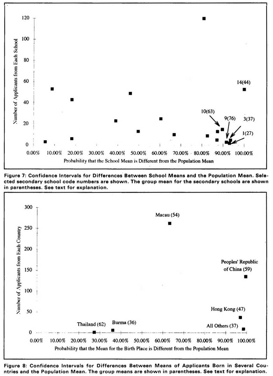
There are 18 secondary schools and 18 corresponding mean values. For each of these values we calculated the probability that the sub-group mean was different from the population mean as described in detail in the Methods section. The proportions of area (formatted as a percentage probability: 100%=total certainty) for the 18 schools and the size of each sub-group (n) were plotted with n on the vertical axis and the probability on the horizontal axis. The sample size is plotted vertically in order to show the sub-groups with small sample sizes more clearly in view of the “nearly normal” nature of the population distribution. Figure 7 shows this plot for the secondary school calculations. Each point was labelled with the school code and the mean for the sub-group in the format, x(y), where x=schools code and y=mean for that sub-group. From Figure 7 we see that for 5 schools out of 18 we can assert with some degree of confidence that their sample means differ from that of the population. These schools fall within the 90% probability interval. The decision to lable these differences as significant or highly significant would depend on the type of question one is asking or other factors. For the purposes of this paper it is sufficient to note these differences. With regard to the population being studied here, we can state that secondary school means vary from 27 to 76with applicants from 5 schools showing that variation. Individual schools are not identified on this graph in order to preserve the confidential nature of information on the application forms. Also it should be recalled that these results have no relation to the curricula at individual schools. They are only relevant to the applicants who took the examination, which is not a proper random sample of the student populations at those schools.
Figure7.
Birth Place
The places of birth included in the data base were Macau, Hong Kong, the Peoples' Republic of China, Burma, Thailand and all other countries. The numbers of applicants in each of these subgroups and the degree of confidence that their sub-group means differ from the population mean is shown in Figure 8. The sample means of applicantsborn in Hong Kong and in all other countries were found to be lower than the population mean (47 and 37, respectively). In contrast, the sample mean of applicants born in the Peoples'Republic of China was found to be higher than the population mean (59). In analyzing the data on performance in the first year and on the Entrance Examination, we noticed a correlation which may be of some interest. First consider the sub-group of applicants who took the examination twice (2-timers). 42 out of 96 of these applicants enrolled in the University. When we examine the performance of the whole group and of the group who
Figure 8.
became students on the Entrance Examination sub-divided by place of birth we see that both the applicants and the students who were born in the Peoples'Republic of China stand out sharply from the rest as having higher mean scores on both Entrance Examinations. These results are shown in Table 6. In doing these calculations, the reference group for comparison was always taken to be the mean and standard deviation of the group of all 2-timers as a whole;be that applicants or students. For example, the reference group for the value 94.9% for the P.R.C.2-Timer Applicants is 53.8, the value for All2- Timer Applicants. All probability value greater than 90% are shown in bold face type. The mean values for applicants in the All Other 2-Timer Applicants category are very low however, the sample size is also very small. Therefore, these results must be viewed with some skepticism. (None of these applicants enrolled as students so they are not shown in the second half of Table 6.) In addition to higher absolute mean scores for the PRC group of applicants, this group also achieved an average increase of 14.7 points by repeating the examination as compared with 12.8 for the population mean of all students who repeated.
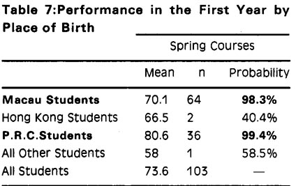
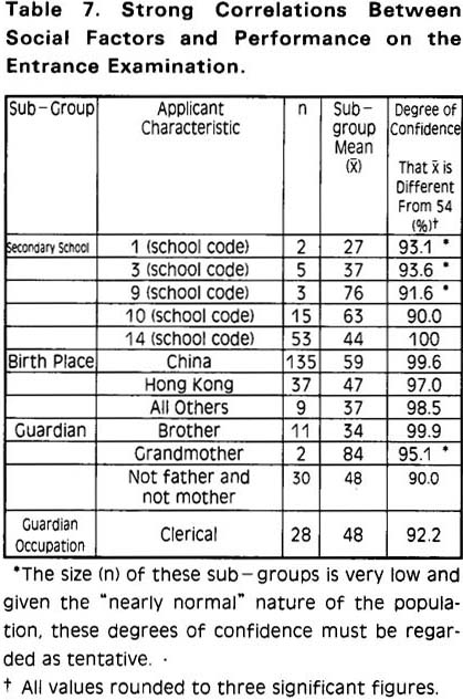
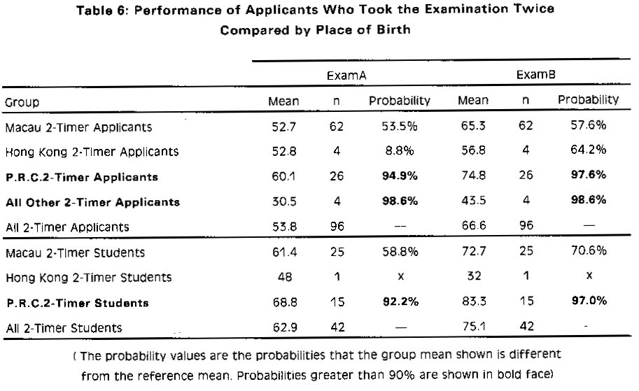 When the performance of students in first year courses were examined by place of birth again the students who were born in the Peoples' Republic of China had a group mean score in the Spring maths courses significantly higher than the reference group (all students in the Spring courses).(Table 7) In addition, we see that the students born in Macau had a group mean score in Spring maths courses significantly lower than the reference group. Since the reference group is made up of essentially Macau students (64 out of 103) and PRC students (36 out of 103) these results may mean than the class of 1990/1991 was composed of two distinct groups as regards mathematical competence.
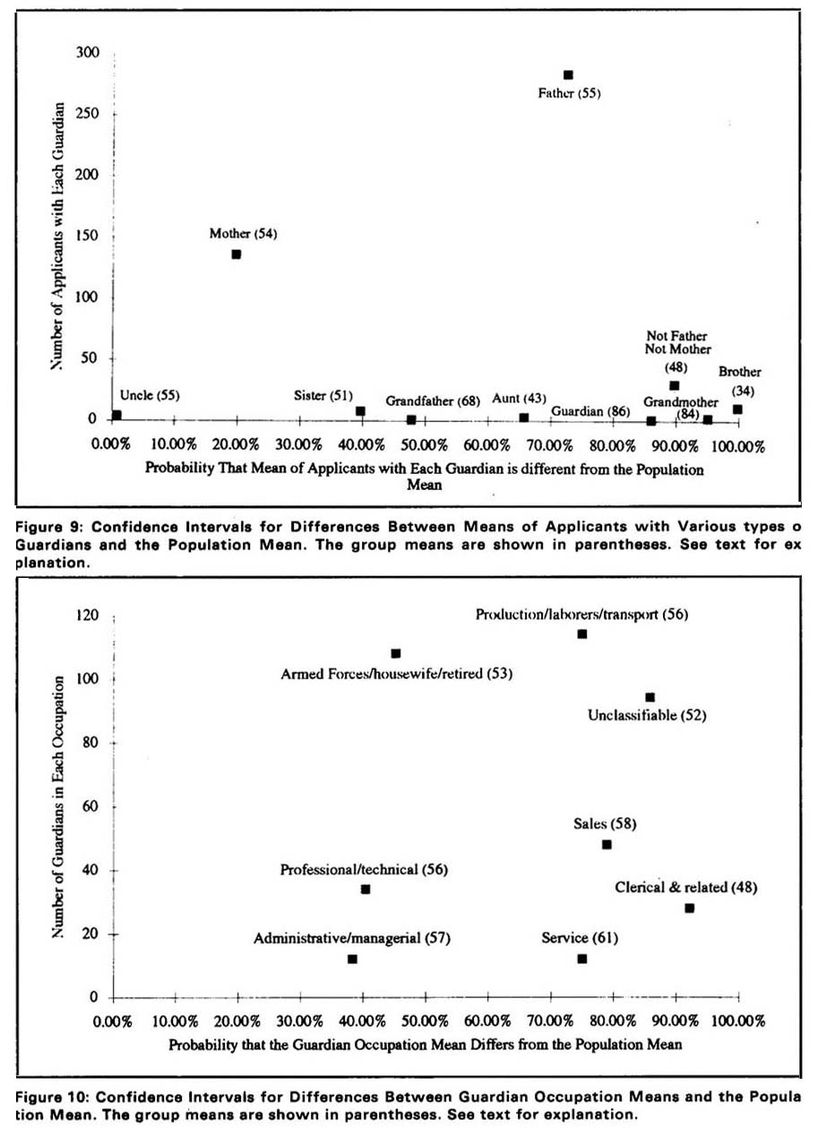
Relationship of the Legal Guardian to the Applicant.
The applicants in this study identified their legal guardians as father,mother,sister, brother,aunt,uncle, or grandmother(subgroups with n>1).ln Figure 9 we show the data plotted in a manner similar to the plots of Figures 7 and 8. Applicants who listed their guardian as father or mother performed similarly to the population as a whole. Applicants who listed their guardian as someone other than father or mother achieved a mean examination score of 48 (n =30) which lies in the 90% probability interval regarding its difference from the population mean. This may be of significance, especially since two classifications within this subgroup, aunt and brother,exhibit very low means (43 and 34, respectively)--although another member of the subgroup, grandmother, has a very high mean (84). The numbers here are quite small, so it may not be wise to make much of these differences, even though ,statistically speaking ,they appear to be quite significant.
Figure 9.
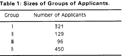
Occupation of the Guardian
The question on the application form requesting the occupation of the guardian was of the open-ended response type:applicants simply wrote a word or words descrbing their guardian's occupation. This question was seriously flawed for the purposes of our study. The question should have been designed with several standard answers corresponding to the classifications which are appropriate for this area and type of study. Accordingly, we classified the responses to the best of our ability into the standard classifications already discussed (see Table 2Methods). However, this classification was very difficult to do in the case of many of the responses. One word used very frequently was “housewife” when the guardian was “mother”.This designation is not descriptive of the guardian's education, skill level, or other factors which can be more easily determined from standard occupational classes. In addition, the term “housewife” may not distinguish the guardian from “mother”sufficiently to separate the clearly very real sub-factors affecting applicants listing this class of guardians. Figure 10 presents the results for subgroups classed by guardian's occupation. We see that the applicants whose guardians worked in the occupation “Clerical”exhibited a low sample mean which may be significant.
Figure 10.
DISCUSSION
Examination Papers
The data of Figures 1, 2and 3 indicate that the only one applicant (from the second sitting) received a score in the range of O to5 and that no applicants received a score in the range of 95 to 100. This means that the examination papers were neither too difficult nor too easy for the population of 450 applicants. Therefore, the score on the papers should be a fairly accurate measure of the competencies of the applicants to solve the problems in the topic areas presented in a testing situation. The fact that such a large percentage of those who repeated the examination were able to increase their score (>85%)is a little disturbing and probably is worthy of further work in the interest of making a fair and unbiased examination paper.
The Population Examined
The two groups of applicants who took the examination only once are very different. Group I (See Figure 1) has scores that are normally distributed whereas Group Ⅱ (see Figure 2)is broken into two sub-groups. Although the mean scores for the two groups are essentially identical, the distribution of Group Ⅱ's results is broader than the distribution for Group Ⅰ. If the two subgroups (Figure 2) are not mere statistical artifacts, then these results suggest that some applicants who took the examination for the first time at the second sitting were less well prepared (Sub-group Ⅱ a centered on scores 26-30) and others were better prepared (Sub -group Ⅱ b centered on scores 71-75) than the applicants who took the examination on the first sitting (mean 54.3). In understanding these results, we need to keep in mind the fact that the two examination papers were different;even though care was taken to make them as similar as possible. One possible explanation for the existence of Group Ⅱ b is that many applicants who wanted to take the examination on the first sitting also were taking another examination in Hong Kong on the same day. It has been suggested that this group of applicants were among the best students of the graduating classes in Macau. It is impossible to assess the truth of this suggestion owing to the lack of information. Even if it were true, it does not explain the comparatively low scores of the other sub-group (Ⅱ a--Figure 2).
The group of applicants who repeated the examination is an interesting one. 57 out of 96 applicants received a passing score or better (>50%) but elected to retake the examination. Of course, the applicants did not receive their grade reports prior to the second examination so it might be argued that some of them repeated it “just to be sure”. However, there were 20 out of the group of 96 who scored>70% and retook the examination. In addition, of the 96 who repeated, 10 actually experienced a reduction in their score compared to the first try. These results are consistent with the conclusion that the applicants who elected to repeat the examination were a random sample of the ones who took it the first time. If this is so ,then we are immediately faced with the question, What could have been their motivation for repeating the examination?
The distribution of Group Ⅰ scores (Figure 1) is clearly normal. When combined with Group Ⅱ, however, the resulting population (Group Ⅳ, Figure 3) is not strictly normal. The histogram of Figure 3 shows that the fit to the normal curve is only approximate and the x2 test confirms this observation. The demonstration of normality for the population under study is crucial if one wants to assert with confidence that sub-groups of the population with fewer than 30 members have means that are significantly different from the population mean. If the sample size is less than 30 and the population is not normally distributed then the sampling distrbution of the means is not normal and the conclusions based on comparing means and confidence intervals would, therefore, not be valid. However, if the population is normally distributed, then the sampling distribution of the means will be normal for all sample sizes and the comparisons will be valid. Some of the large differences from the population mean observed for sub-groups were for very smallsample sizes and so given the “nearly normal”nature of the population, we must be cautious about drawing conclusions for these small sub-groups.
Using the Entrance Examination as a Basis for Admissions Decisions
The scatter plot and correlation coefficients presented under Results( Figure 5 and Table 4) represent an attempt to determine if the score on the Entrance Examination is in any way correlated with the students' performance in the first year courses. Our findings agree with those of investigators in the United States who examine the correlation between the scores received by applicants to US universities on the Scholastic A ptitude Tests (SAT) and the overall GPA (grade point average) in the first and sometimes subsequent years of the students' academic lives (for review see Kanarek, 1989). The degree of correlation between these two statistical variables is very low. We do not regard correlation coefficients of 0.2 to 0.6 as meaningful even if they can be shown to statistically different from zero (Kanarek, 1989).The data shown in Figure 5 have a correlation coefficient of 0.52. This would seem to indicate that there is some relationship between a student's score on the Entrance Examination and his or her grade in the first year maths course. On the other hand, consider the applicants (whose scores appear in Figure 5) who had low Entrance Examination scores but, once admitted, scored very well in their first year maths courses. Also, there are many applicants for whom the converse is true (Figure 5). Therefore, it seems inappropriate to use the Entrance Examination as a measure of how well applicants will do in University programs; that is, as a predictive measure of possible success in the first year. On the other hand, some sort of examination in a specific topic, like maths, could be useful in determining if applicants have learned a minimum prerequisite body of knowledge necessary for entering university study and standardizing the level of knowledge required. This topic is quite controversial in the United States currently (Kanarek,1898;Breland et al., 1982;Merante et al., 1983, Willingham and Ramist,1982). The investigations focus on what indicators in the academic life of a secondary school student should be used in making admissions decisions.
A university admissions committee should be seeking answers to both of the following questions in making admissions decisions about applicants. (1.) Has the applicant learned the body of knowledge tested for well enough to use that knowledge in a more advanced context in order to go further in that same field of knowledge as required by the standards of the university programs?ln short, is the applicant ready for more advanced study in that field?(2.) Will the applicant be able to succeed in the courses required by the majors of the university which s/he could choose once admitted and will the applicant ultimately be able to finish the four year program with a bachelor degree. Answers of Yes to both questions should be required in the case of a decision to admit an applicant. The second question is focused on the commitment of the applicant to achieve a bachelor degree. This commitment is distinct from readiness to pursue a course of study, which is the focus of the first question. A prospective student who has learned a body of knowledge well may or may not be committed to going further even though s/he thinks that s/he has made a decision which is right for him or her. The reason for this is that a student's decision to apply for admission and seek a higher degree is not necessarily governed by his or her intrinsic desire to do so. Other factors like family and societal pressure may influence a student sufficiently to “force”him or her to apply and to do well on an entrance examination, when, in fact, the student actually wants to be doing some other type of activity. Such a student has little true commitment to the scholastic endeavor. Conversely, a prospective student may be absolutely clear about his or her de-sire and commitment to pursue a university degree but if the basic or prerequisite knowledge has not been obtained before entering that path, then success is doubtful. The reasons that these questions are central to admissions decision have to do with considerations which should be of great interest both to the applicant and to the university.
For the applicant, the academic pathway leading to a bachelor degree is usually four years of time spent in an endeavor which, at times, it must be admitted, seem far removed from more practical problems related to living and survival. Also, there are strong emotional factors present which are connected with growing away from a small -world of teen-age friends and family life to a larger one of independence and responsibility for one's own actions. For a student to stay with such a program in the presence of the many divergent and, at times, confusing forces, s/he must have a clear vision of what may be possible afterwards and clearly be dedicated to having that vision in his or her life. If such a vision is not present, then the probability that the student will succeed and finish the program is low. Thus, a negative answer to the second question cripples the student who is admitted anyway from the outset of the program and threatens to waste the time and money s/he spends in such an endeavor which could have been spent more profitably in another area. So the student has four years of time and a good deal of money to lose if the decision to admit is made incorrectly by not considering the second question above. Consideration of this question should be made by both the applicant and the university. An entrance examination cannot measure or even address the question of an applicant's commitment to pursue a bachelor degree. Determination of this factor must be obtained by other measures in the applicant's backgrounds.
For the university, a yes answer to both of these questions will provide students for the university programs who are eager to learn and well prepared. Among such students, the probability of there being brilliant, creative individuals who will do honor to the university and magnify the name and standing of the university in the community and in the world is great. The attrition from programs will be low and larger fractions of graduating students will seek advanced postgraduate degrees than if students are admitted whose preparation and commitment to study are minimal or questionable. Ultimately, admitting committed, well prepared students enhances all programs by raising the level of the academic endeavor. Also, the programs function more efficiently since special cases are minimized and course failure rate is low. Since a large proportion of students receive substantial financial aid subsidies for their tuition, this money is used more efficiently too by accepting well prepared and committed students than by accepting students whose preparation and commitment are questionable. Finally, staff morale is improved since the instructors deal with a more consistently achieving group of students who genuinely want to learn, are ready to do so and therefore can interact more creatively with instructors than students whose presence in the classroom is marginal at best.
This discussion raises the question of how to identify those students who are both committed and well prepared. It is this very problem about which much of the discussion in the United States is currently centered. Most investigators agree that using a single variable like admission examination scores on which to base admission decisions is a very poor way to address these problems (Kanarek, 1989; Merante, 1983;). Universities which are focused on obtaining students with high probabilities of finishing their programs successfully use a multiple factor approach in which SAT scores, secondary school GPA, letters-of recommendation, extracurricular activities, or other accomplishments of the applicants are considered to “predict” a most likely minimum GPA in the first year. These universities then set somecut-off point for accepting applicants based on the “first year predicted GPA”. The theoretical basis of this approach seems valid: SAT scores measure competency in certain basic academic subjects. Secondary school GPA measure overall performance over a period of time similar to that contemplated for the achievement of the bachelor degree. In combination with extracurricular activities, a reasonable GPA shows an ability to deal with multiple forces simultaneously in addition to having a component involved in commitment to the academic program. Thus, the multiple factor approach seems to address at least some of the factors alluded to above as being crucial to admissions decisions. In fact, such a system of decision does produce groups of students who generally do well and finish the programs with minimum attrition.
Examination Performance and Age.
These results (shown in Figure 6) are quite striking and indicate that younger applicants did better on the Entrance Examination than older applicants. One explanation of this result is that if older applicants have been out of school for a longer period of time than younger applicants. We have no way of testing this hypothesis in this study. We should note in passing that the correlation shown in Figure 6 would not be so obvious if the method of confidence intervals were used to determine if differences in sample means from the population mean were significant. Such differences are only significant for ages 19,20,23 and 25. The reason for this is possibly that the line of the subgroup means passes through the value for the population mean (between ages 20 and 21). Thus as the sub-group means approach the population mean their individual differences become very small and not statistically significant. However, we can see from the strong linearity of the least squares fit shown in Figure 6, this correlation is one of the strongest found in this study.
Examination Performance and Social Factors.
Of the social factors we were able to work with (sex, secondary school, birth place, relationship of the guardian and guardian occupation) the strongest correlations observed with examination performance are the ones shown in Table 7. For these subgroups the degree of confidence that the sub-group mean is different from the population mean is above 90%.
The applicants from the 5 secondary schools in Table 7 exhibit a very broad range of mean scores (27 to 76). The applicants who were born in China present an intriguing group. The group is large and the difference in their mean score from the population mean in highly significant. Examination performance is especially outstanding for applicants born in China who took the examination twice. It is even more interesting to note that apparently these applicants were educated in Macau. What part of that education may have occurred here cannot be determined from this study. However, these students stand out prominently from the others in the population. It would be of great interest to examine this group more closely.
Applicants who listed their mother or father as their guardian appear to have constructed the mean (n=420 compared to N= 450 for the population). The degree of confidence for the means of the applicants who listed brother and grandmother are very high. However, we question the validity of these data. The reason for this doubt has to do with a cultural bias toward not revealing too much personal information about the family. Thus in some families perhaps the father (or mother as breadwinner) declined to be listed on the application for personal reasons. For example, 69 out of 450 applicants declined to list the guardian's occupation. We have no way of assessing the contribution to these data from false responses such as these, but we simply note that the possibility of corrupted data may exist and leave it to further studies to find out if sucha problem exists.
Examination Performance and Sex.
The fact that there is no correlation between sex of the applicants and mean scores on the entrance examinations of either the first or second attempts would seem to point to a degree of equality in the education standard for boys and girls. This result is interesting particularly since boys are given psychological and cultural advantages in Macau society. Any hypothesis to explain this outcome would be mere speculation since in our data base is no information to address this question.
REFERENCES
Breland, H.M.et al. (1985) Research Report of the Educational Testing Service. (Princeton, NJ). “An Examination of State University and College Admissions Policies”.
Kanarek, E.A.(1989) Paper presented at the Annual Forum of the Association for Institutional Research. (Baltimore, MD, April 30May 3 1989). "Exploring the Murky World of Admissions Predictions".
Merante, J.A.(1983) NASSP Bulletin. Vol. 67.No. 460. Pages 41-46. “Predicting Student Success in College”.
Wileman, S. et al. (1982) Journal of Computers in Mathematical and Science Teaching. Vol. 2. No. 1. Pages 20-21. “The Relationship Between Mathematical Competencies and Computer Science Aptitude and Achievement”.
Willingham, W.W. and Ramist, L. (1982) Phi Delta Kappan. Vol. 64. No. 3. Pages 207208.“The SAT Debate: Do Trusheim and Crouse Add Useful Information?”.