Computer Simulation of Heat Treatment Transformation Processes
C.C. Szilvassy (Faculty of Science and Technology, University of Macau) M.Gergely,and t.Reti (Technical University of Budapest,Hungary)
在不同的熱能處理中,電腦模擬與預測鋼在不同的溫度下動能的轉變,具有重大且實際的重要性。
本文關於電腦模擬的基本目的,包括:模組敍述,動能轉變模式,和相對微型結構特質。計算微型結構與特性,可利用下列十三個模組:決定martensite,計算熱能曲線,計算到 austenisation 的時間和溫度,計算austenite grain size,計算TTT圖表,計算冷凍曲線,持續冷凍轉變模式,微型結構轉變的決定,堅硬度的計算和溫度電腦模組。
Industrial Summary
Computer simulation and prediction of transformation kinetics in steels at varying temperatures are of great practical importance in different areas of heat treatment.
This paper deals with basic objectives of computer simulation; the model description, the modeling of transformation kinetics and the relating microstructure to properties; calculation of microstructure and properties using thirteen modules: determination of martensite,computation of heating curve, calculation time and temperature to austenisation, computation of austenite grain size, calculation of TTT diagram, computation of cooling curve, modeling of continuous cooling transformations, determination of microstructural transformations, calculation of hardness, and tempering computer model.
1. Introduction
COMPUTER SIMULATION is a method of computer application that is expected by heat treaters to yield great results in the future. In recent years, the establishment of prediction methods based on the phenomenological description and computer simulation of the transformation processes during heat treatment and the development of software for technological planning have been of major interest. The steady development of this topic is aimed at meeting the requirement of metallurgists producing basic materials, design engineers dealing with material selection and dimensioning, and technologists planning heat-treatment processes. In this article, the topic of computer simulation is restricted to quenched and tempered or case-hardened steels.
2. Basic Objectives of Computer Simulation
The development of computer simulation of heat treatments, which is obviously due to the widespread growth of computer miniaturization, has been motivated by several factors. Research in this field of computer simulation has been concentrated so far on two main areas of interest:
# Modelling of transformation processes and the prediction of microstructures and/or properties.
# Developing program packages (designed in the majority of cases to be purchased on the market for direct industrial use) to help solve concrete tasks such as material selection, property prediction, andthe design of heat-treating operations.
3. General Concept of a Property-Prediction System
A detailed Property-Prediction System (PPS) used for simulating the metallurgical process occurring during heat treatment and predicting the microstructure and mechanical properties of quenched and tempered or case-hardened steels is described in this section. The system consists of several modules, which form a logical chain for property prediction.
3.1 Model Description
Before starting to design a PPS, one has to ascertain first those internal parameters (for example, Ac3 temperature, transformation kinetic data, hardness values of the microstructural elements, and so on) that have the most determinative effects on the properties. Then the algorithm, the logical chain of these internal parameters, has to be stated and finally, the connections between the input data, the internal parameters, have to be investigated. If all of these connections are clear, mathematically formulated, and joined into a chain, one can handle this set of connections as a system.
This programs of the PPS are based on a phenomenological model of kinetics of transformation taking place in nonisothermal conditions. The program permits the prediction of the progress of transformations, of the microstructure, and of the mechanical properties as a function of time and of position in the cross section of the heat-treated workpiece. The equations forming the base of the model belong to three main groups as follows:
# The differential equation of heat conduction : By a numerical method, the temperature field in the given workpiece is solved.# The system of kinetic differential equations for describing the transformation processes occurring in the microstructure.
# Equations describing the relation between the microstructure and properties.
3.2 Modelling of transformation kinetics
Modelling of transformation kinetics can be done with differential equations such as:

where t denotes time, r is the vector representing a given point of the workpiece (the position vector); T is the temperature, which is a function of time t and position r ; Yj (j = 1, 2,... J) is a so-called microstructural parameter; and gj = 1, 2,... J is an appropriately selected real value function.
The microstructural parameters Yj in Eq 1 are numerical quantities that may be interpreted within relatively wide limits. For example, Yj may denote the volume fraction of the transformed phase, its average dimension, or the mean free distance between particles.
3.3 Relating Microstructure to Properties
The starting point for predicting mechanical properties such as hardness and yield point is that the properties are related to microstructural parameters. It was assumed that after transformation at a given location r in the workpiece, a numerical property P(r) of the steel may be calculated with a precision satisfying practical demands as a function of a small number of elementary microstructural properties Pj (j = 1,2,...M) according to the formula:
P(r) =f1(P1,P2,...PM) (Eq 2)
where f1 is an appropriately selected function.
In most cases, the so-called generalized linear law of mixture represented by the following Stieltjes integral was used to calculate the elementary microstructural property Pj (j = 1,2,... M):

where x [ T (r, t), Yj] is a suitably defined weighting function containing and summarizing the numerical information on the given property of the microstructural parameter Yj.
4.Calculation of Microstructure and Properties
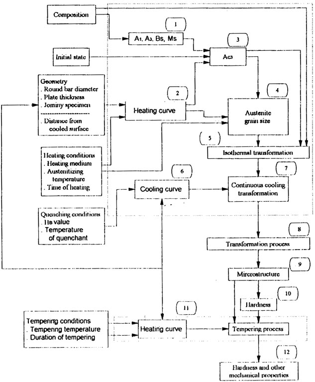
The block diagram of a PPS program is shown in Fig 1. The upper part the diagram refers to the processes occurring during austenitization and quenching; the lower part refers to tempering processes. The "black boxes" of the quenching and tempering calculation unit are within the frames shown with dashed lines. The programs that form the system are numbered 1 to 12. The models and the parameters used as input to the modules are being developed continuously according to the latest experience and can be changed. Each module is described in this section.
The input data are seen on the left side of the block diagram. They are as follows:
# Chemical composition of the workpiece to be hardened
# Initial state of the workpiece (annealed, normalized, quenched,
  and tempered)
# Geometry: shape and size of the workpiece (round bar or plate)
  characterized by its diameter or thickness, or Jominy specimen and
  the distance from the cooled surface to the point where the
  microstructure and properties are to be predicted
# Heating conditions: heating medium, austenitizing temperature,
  and the total time spent by the workpiece in the austenitizing
  furnace
# Quenching conditions characterized by the HB value (relative heat
  transfer coefficient specifying the cooling severity, for example, in
  the case of oil, 0.3 to 0.6) and the temperature of the quenchant
# Tempering conditions given by the tempering temperature and the
  duration of tempering
4.1 Determination of Martensite Start(Ms), Bainite Start(Bs), and the Equilibrium (A1, A3) Transformation Temperatures from Composition (Module 1).
The chemical composition of the workpiece is first verified against the specified composition range of the steel type for which the predictor program was developed. From the composition, Module 1 then calculates A1, A3, Bs, Ms transformation temperatures by formulae based on dilatometrical measurements and regression analysis. There are also numerous formulae in the literature for the estimation of these transformation temperatures [1].
4.2 Computation of the heating curve (Module 2)
Computation of the heating curve (Module 2) takes into account the furnace features. Calculations are based on the application of an approximate method developed to solve heat conduction problems for simple geometries.
In most practical cases, it is not necessary to expend much effort for the accurate calculation of the heating curve. The accuracy of the following Newtonian approximation can also satisfy the requirements:
T=(To-Ta)exp{ -aht} + Ta (Eq 4)
where T is the temperature in the given point of the workpiece; t is the time; Ta is the austenitization temperature; To is the temperature at t = 0; and ah is a constant, depending on the furnace, mass of workpiece, heating medium, quality of the surface, and agitation of the medium.
4.3 Calculation of Time and Temperature to Austenitization (Module3).
This module calculates the austenitizing temperature (Ac3) to the nearest 20℃ (35°F) and the time to reach the Ac3 temperature. The Ac3 temperature is determined--apart from the chemical composition--by the initial microstructure and the heating rate. The interactive computer program based on this model permits the user to select one of four of initial microstructures. The experimental results may be described with the following equation:

where v is heating rate at temperature A3, and a is a parameter depending on the initial state of microstructure, that is, the finer the microstructure is, the lower the value of a. The value of the empirical parameter a is estimated by least squares analysis on the basis of grain growth diagrams of different steel grades (see Fig 2 and the corresponding discussion of grain growth given below).
For the chromium-molybdenum low-alloy steels with 0.5% C content, the numeric value of the a parameter can vary from 3 to 15, if the temperature are measured in degrees centigrade. For example, in the case of a quenched microstructure, a = 3; for quenched and tempered state, a =5; for the normalized state,a = 10;and for the annealed state, a = 15.
4.4 Computation of the heating curve (Module 2)
Computation of the heating curve (Module 2) also requires consideration of nonisothermal conditions. The extent of grain growth taking place during austenitization is known to have a decisive effect on the characteristics of steel; therefore, its prediction is a task of considerable practical interest [2].
Grain growth diagrams were worked out for the various types of steel on the basis of tests, but their usefulness was restricted by the condition that they must be valid for the case of isothermal or linear heating. It was shown [3] that using the data of the known austenite grain growth diagram valid for linear heating, a generalized kinetic function can be produced by calculation, which allows computed tracking of grain growth taking place at changing temperature, and thus prediction of grain size.
It was assumed that grain size Da of steels at constant temperature Teis described by an isothermal kinetic function of the following type:

After derivation, the generalized kinetic differential equation type (Eq 1) is obtained:

The unknown parameters ko, N and Qa of differential equation (Eq 7) can be estimated by regression analysis using measured data*. According to the published method [3], the average grain size Da may be calculated with the generalized kinetic function:

produced by integration of the generalized kinetic differential equation (Eq 7). Knowing the heating curve, the solution can be obtained by numerical integration of Eq 8, where Do is the initial grain size at Ac3; N and Qa are parameters depending on the composition, and R is the universal gas constant. The values of the parameters ko, Qa, and N may be determined by the method of least squares from grain growth experiments.
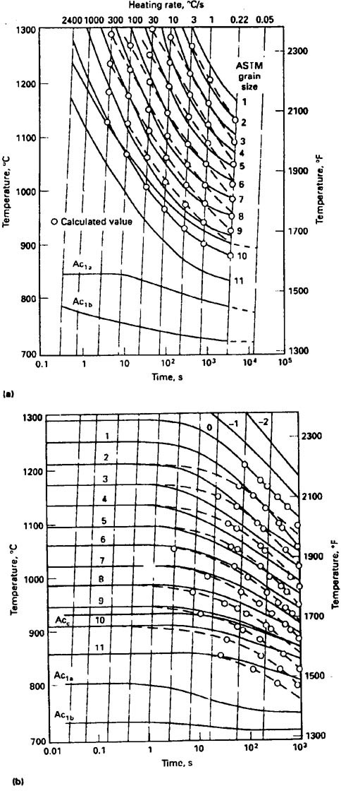
Figure 2 shows two grain growth diagrams for steel 90MnV8 as examples. In Fig 2, the solid lines represent the original test results [4], while the dashed lines show the results calculated with Eq 8. For this calculation, the time-temperature function had to be substituted before integration. The applied parameters were as follow:
ko=6. 087× 10 7
N=2.44
Qa=317kJmol-1
* In the case of steels with grain-refining elements (aluminum. niobium. titanium, and so forth), if the temperature exceeds the temperature of dissolution of second phases (nitrides. carbides). the parameter ko, N, and Qa have to be altered. It must be notedhere that the usual austenitizing temperature is less than the dissolution temperature, which ranges between 970 to 1050~`0C (1780 to 1920~`0F).
Figure 2 (b) shows the grain growth for the same steel but, for isothermal conditions, taking into account the heating rate as well. The coincidence of the grain sizes determined by measurements and those calculated by Eq 8 are satisfactory according to practical demands.
4.5 Calculation of TTT Diagram (Module 5).
The characteristics of the isothermal time temperature transformation (TTT) chart are calculated as a function of the chemical composition and austenite grain size, also taking into account the temperature A1, A3, Bs, and Ms.
A complete mathematical description of the isothermal transformation, starting with nucleation and growth, is presently not possible for large volume fractions transformed [5], [6]. The reason is that an analytical description of the growth is not possible if the single nuclei touch each other. Therefore, in general, empirical descriptions are used that are appropriately fitted to the measure curves. Some of the applicable methods are listed below.
Avrami Estimate of Isothermal Transformation. One of the most frequently used equations for the isothermal transformation is Avrami's equation:
y = 1 - exp{ - btn} (Eq 9)
where y is the volume fraction of the transformed austenite; t is the time spent on the isotherm; and b and n are temperature, grain size,and composition-dependent constants, evaluated from the isothermal TTT diagram of from measurements with continuous cooling [5].
For calculations detailed below, the parameters b and n can be given in tabulated form, but also in mathematical form as functions of temperature, composition, and grain size.
Estimates of 1% and 99% transformation. The second possibility is to define functions for the beginning (1% transformed austenite) and for the end (99%) of isothermal transformations. These curves can be described with equations of the following form:

Where C is the composition vector; Da is the austenite grain size; T is the temperature; ho, h1, h2 and h3 are composition-dependent constants; and f2 is a suitable selected real function.
Transformation Estimates from Isothermal Kinetic Differential Equations. In the PPS program discussed here, the information content of the traditional TTT charts is built into the program in the form of isothermal kinetic differential equations as follows:

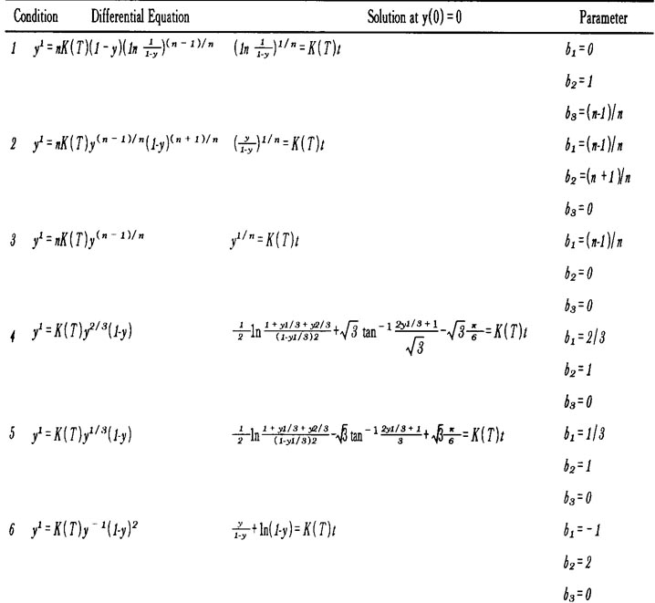
where y is the relative amount of transformed products; K, b1, b2 and b3 are appropriately selected parameters depending on temperature, austenite grain size, and composition [7]. The most important kinetic functions (Table 3) can be considered as special cases of Eq 11.
Table 3 Summary of most important kinetic functions for isothermal conditions
4.6 Computation of the cooling curve (Module 6)
Computation of the cooling curve (Module 6) at the given point of the workpiece can involve a simple method similar to the one described in Module 2, that is, to use a Newtonian cooling:

where Ta is the austenitization temperature; Tq is the temperature of the quenchant; and ac is the geometry and quenchant-dependent parameter.
In the case of cylindrical workpiece and water cooling, the equation for calculating ac can be suggested in the following form:

where D is the diameter; X is the diameter from the cooled surface; and A and B are agitation-dependent constants.
The computer program discussed here takes into account the individual geometry (plate, cylindrical workpiece) and calculates the cooling on the basis of the principles similar to one-dimensional unsteady-state heat conduction, which is formulated by the Fourier differential equation as follows.

where t is time; r is locale corrdinate;T(r,t) is temperature; qv is rate of heat generation due to the austenite transformation; p is density; Cp is specific heat;λ is thermal conductivity;β=0 for the plate; and β=1 for the cylinder.
With the cylinder diameter and the plate thickness equal to 2R, the corresponding boundary and initial conditions are:
At the surface(r=R)with t>0:

At the centerline(r=0)with t>0:
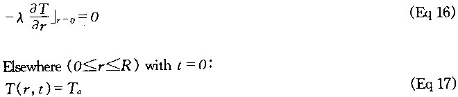
where ais the heat transfer coefficient, Tq, is the temperature of the quenching media; and Ta is the initial austenitizing temperature.
In many cases, the heat generated in the workpiece during cooling is disregarded (qv =0). On the other hand, some simplifying assumptions are used relating to the surface heat transfer represented by Eq 15.
By introducing the relation heat transfer coefficient HR defined as:

then Eq 15 can be rewritten in the form:

The parameter HR (assumed to be constant) is formally equal to the widely accepted quenching factor proposed by Grossmann for characterizing the quenching power of different cooling media [8], [9].
The dimension of HR is the reciprocal of length (l/m, or 1/in). In heat-treating practice, the range of HR is in the interval of 8 to 195 m-1(0.2 to 5.0 in-1), where the 8m-1(0.2 in.-1) is for an oil quenchant without agitation and the maximum value 195 m-1(5 in.-1) corresponds to a brine quench with strong agitation.
Starting with an appropriately selected cooling intensity HR, it is very easy togenerate the cooling curves for the workpiece of cylindrical or plate form. The disadvantage of this model approach is that the value HR is not constant and varies during the cooling process. This fact may lead to computation inaccuracies, which must be taken into consideration.
A more exact and more complicated way to characterize in a quantitative manner the surface heat transfer process during quenching is based on the use of the boundary condition formulated as:

where ¦□is the surface heat flux as a function of the surface temperatureTs. The surface heat flux ¦ can be measure for different quenching conditions (for different quenchants, temperatures, agitations, workpiece geometry, and so forth). It can be stored in a data base and can be retrieved for practical computations [10], [11].
4.7 Modelling of Continuous Cooling Transformations (Module 7).
Calculating the progress of the transformation process during continuous cooling from the TTT characteristics is a crucial part in property prediction. Estimation of the ferritic, pearlitic, and bainitic fractions during each step is based on published methods.
The principle of the method is described below.
In the frist step, the isothermal kinetic differential equation is appropriately generalized in the form:

where T = T(t) is the temperature as a function of time, and f3 stands for a selected real function. In the second step, this equation is solved by a numerical method known as the recursive algorithm. The extension and generalization of this method was published in [12], [13].
The recursive algorithm for the well known Avrami Kinetic function was first formulated by M. Gergely [14]. The volume fraction of ferrite-pearlite and bainite are evaluated according to the Avrami expression defined by Eq 9. The cooling curve is approximated by a staircase, and the transformation is then calculated isothermally during each time step. The recursive algorithm is actually a special numerical procedure for solving the generalized kinetic equation (Eq 21). The verification of this is published in [7].
For the calculation of the amount of martensite, a novel formula is used instead of the well-known equation proposed by Koistinen and Marburger [15]. The martensitic transformation can be described in the following differental form:

where ym is the relative amount of martensite transformed from austenite; and Km, a1, a2, and a3 are composition-dependent parameters.
4.8 Determination of Microstructural Transformations (Modules 8 and 9)
Information about transformation temperature definitions for the initiation of the ferrite-pearlite reaction and for the beginning temperature range, Bs, of the bainite reaction is first provided by Module 8. In practice, the beginning is defined as either 1 or 5%. Actually, the complete transformation curve is available as one of the outputs for further evaluation. On the basis of this curve, the temperature belong to 5%, 10%,... 50%, ... 95%, and the quantities ofthe microstructural elements can be displayed. Module 9 gives the microstructure, namely, the amounts of ferrite-pearlite, bainite, martensite, and retrained austenite, The program uses definitions given above, for example, bainite is the transformation product obtained from austenite between the temperature Bs and Ms.
4.9 Calculation of hardness (Module 10).
When the hardness after quenching is calculated on the basis of microstructure and the carbon content, many investigations are still necessary to ascertain the best rule of mixing. In the Creusot-Loire system [16] the hardness at room temperature of martensite, bainite, and ferrite-pearlite is calculated seperately talking into account the chemical composition and cooling rate at 700℃ (1290℃ ). Then a linear mixing rule is applied to get the final hardness.
The PPS model discussed in this section predicts the hardness by the help of the individual isothermal hardnesses of the microstructural elements. As mentioned in the description of Module 7, the solutions of the differential equation( the recursive formulas) trace the nonisothermal phase transformation. Consequently, in the calculation of the hardness after quenching, the transformed amounts of austenite on each isothermal step, and their individual isothermal hardness can be taken into account. The amounts of the microstructural elements are calculated by the help of the stepwise method. This individual hardnesses of the microstructural elements are taken from a hardness-temperature table or function valid for the actual steel, and the resultant asquenched hardness Hq is composed from these components with the formula:

where Ti is the temperature of the ith step; yi (Ti) is the transformed amount at temperature Ti; H (Ti) is the isothermal steps, until temperaturereaches Ms; ym is the volume fraction of martensite; ya is the volume fraction of retained austenite; Hm is the hardness of martensite; and Ha is the hardness of retained austenite.
4.10 Tempering Computer Model (Modules 11,12, and 13)
Module 11 computes the heating curve to reach the tempering temperature. Modules 12 and 13 calculate the final hardness after tempering according to the published method [ 3 ], together with the prospective tensile strength, elongation, reduction in area, and impact energy.
The tempering of steels forms a significant part of practical heat treatment, and therefore its study and mathematical description are of greatest importance. Several generally applied methods are available for the isothermal case (see the discussion of the Creusot-Loire system in [16]). In the PPS model discussed here and other systems doing mathematical simulation, the calculation of hardness as a function of time with continuously changing temperature has to be solved. From computational considerations, it is assumed that the kinetic equation describing the change in hardness under nonisothermal conditions is of the form:

where Ht stands for the instantaneous hardness after tempering; f4 is a suitably selected function; and Pg is the so-called generalized time-temperature parameter, which is applicable to the description of tempering processes with changing temperature.
The form of the parameter Pg can be selected in many ways. For example, the generalized version of the widely used Hollomon-Jaffe parameter is:

where C is a composition-dependent constant. It follows from Eq 25 that if the tempering temperature is contant, that is, T = Tc, the conventional Hollomon-Jaffe parameter.

is obtained as a apecial case.
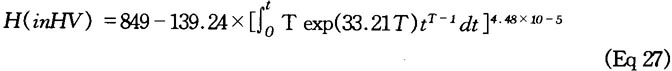
As an example for an unalloyed steel containing 0.6% C, the kinetic equation that is valid for continuously changing temperature and describes the changing Vickers hardness (HV) of martensite during tempering is as follows:
Using this method, a microprocessor-bs aed system can be designed that continuously displays the instantaneous value of the required characteristic (for example, hardness), from measurement of the actual temperature of the piece during heat treatment. When the preset hardness value is achieved-using the programmability of the processor-a variety of interventions can be made to the heat-treatment process.
From Eq 24 a new type of tempering chart, of more general validity than before, may be obtained. This case used the generalized Dom parameter defined as:

The tempering chart (Fig 3) is composed of two independent parts. Thelower part of Fig 3 refers to isothernal heat treatment and shows the relationship of tempering parameter PD to temperature and time. This chart can be applied to convert from one tempering time and temperature to any other, on the basis that combinations of tempering temperature and time having the same value of tempering parameter will produce the same hardness. The upper part of Fig 3 represents the relationship between parameter PD and the tempering hardness for 50CV2 steel (0.5%C, l%Mn, l%Cr, 0.15%V).
For tempering at varying temperatures, the value of the parameter PD required to achieve the specified hardness may be determined with the aid of the upper part of Fig 3. For isothermal tempering, the various time-temperature combinations for the given parameter value PD, which may be used to achieve the specified hardness, may be read from the lower chart in Fig 3.
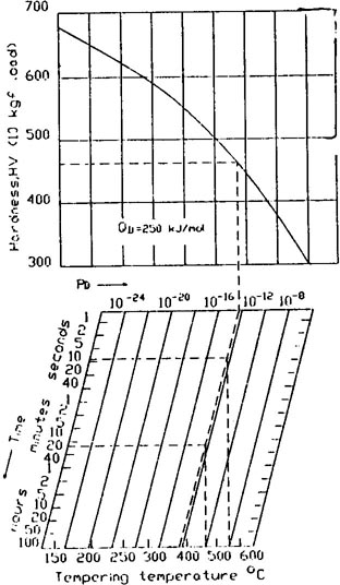
In the kinetic function employed for the phenomenological description of hardness decrease occurring during tempering, The value of the apparent activation energy (QD = 250 kJ/mol) is essentially identical to the activation energy for the self-diffusion of ferrite in steel that is not alloyed with molybdenum. However, the upper chart representing the so-called master curve must be deduced and plotted individually for the various steel types from measured data.
4.11 Mechanical Property Estimates.
Module 12 estimates not only the hardness, but also the other mechanical properties, namely the tensile strength, yield strength, elongation, reduction in area, and the Charpy value of the impact energy with the following formulas*

where Rm is the ultimate tensile strength in MPa, and HV is the Vickers hardness.
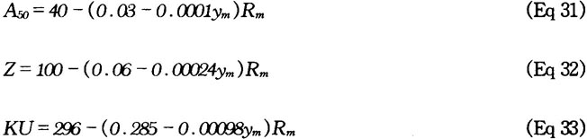
For the calcution of the yield point R (MPa), elongation A50(%) in 50 mm (2 in.), reduction in area Z(% ), and Charpy value KU(Joules), the equations below have been suggested:

where ym is the volume fraction of martensite in%.
There are some other possibilities developed by utilization of the data base of individual steel properties.
References
[1] T.Ericsson. Ed., Computers in Material Technology, Proceedings of the International Conference, Linkoping University, Pergamon Press, 1980, pp 3-68
[2] M. Gergely, Mathematische Beschreibung des Austenitkornwachstums bei Isothermen Bedingungen und bei Temperaturanderung, Neue Hutte 21 (12) (1976) 725-727
[3] T. Reti, G. Bobok, and M. Gergely, Computing Method for Nonisothermal Heat Treatments, Heat Treatments 81, The Metal Society, 1983, pp 91-96
[4] J. Ohrlich, A Rose, and P. Wiest, Zeit Temperatur -Austenitisierung - Schaubilder, Atlas zur Warmebehandlung der Stahle, Band 3 Verlag Stahleisen M. B.H., 1973
[5] G. Buza, H.P. Hougardy, and M. Gergely, Calculation of the Isothermal Transformation Diagram from Measurements with Continuous Cooling, Steel Res., Vol 57,12(1986) 650-653
[6] T. Reti, M. Gergely and C.C. Szilvassy, Property Prediction ofQuenched and Case Hardened Steels Using PC, IMMA Conference 1991, Materials Processing and Performance, Australia, 1991, Vol 2.pp 257-273
[7] M. Gergly and T. Reti, Application of a Computerized Information System for the Selection of Steels and Their Heat Treatment Technologies.J. Heat Treat., Vol 5, 2 (1988) 125-140
[8] M.E. Dakins, C.E. Bates, and G.E. Totten, Calculation of the Grossman Hardenability Factor from Quenchant Cooling Curves, Metallurgia, Furance supplement, 12 (1989)7
[9] M.A. Grossmann, M.Asimow, and S.F. Urban, Hardenability:Its Relation to Quenching, and Some Quantitative Data, Hardenability of Alloy Steels, American Society for Metals, (1939) 124-196
[10] B. Liscic and T. Filtin, Computer-Aided Evaluation of Quenching Intensity and Prediction of Hardness Distribution, J. Heat Treat., Vo15, 2(1988) 115-124
[11] J. Wunning and D. Liedtke, Versuche zum Ermitteln Der Warmestromdicte beim Abschrecken von Stahl in Flussigen Abschreckmitteln nach der QTA-Methode, Hart - Teah. Mitt., Vol 38,4(1983) 149-169
[12] T. Reti, M. Gergely, and P. Tardy, Mathematical Treatment of Non-isothermal Transformations, Mater. Sci. Technol., Vol 3, 5 (1987) 365- 371
[13] M. Gergely, T. Reti and C.C. Szilvassy, Mathematical Modellingof Transformation Processes during Heat Treatment (Hardening and Tempering) of Steel, Modelling and Control of Materials Processing Conference, Wollongong Australia, 1992
[ 14 ] M. Gergely, Eine Moglichkeit der Berechnung von Hartungsspannungen aufgrund der Unwandlungseigenschaften des Stahles, Hart. Tech. Mitt., Vol 27, 3(1972) 184-186
[15] D.P. Koistinen and R.E. Marburger, Acta Metall., Vol. 7, (1959) 59-60
[16] D.V. Doane and J.S. Kirkaldy, Ed., Hardenability Concepts with Applicationa to Steel, American Society for Metals, 1977,pp 493-496
Fig 1 Block diagram of the PPS simulation model
Fig 2 Measured and calculated austenite grain growth diagrams of 90 Mn V8 steel (0.85 - 0. 95%C, 0.15-0.35%Si, 1.8-2.0%Mn, 0.07-0.12%V) during (a) continuous heating and (b) isothermal heating at 1.3~`0C/s (2.3~`0 F/s)
Fig 3 Generalized tempering chart obtained using the generalized Dom parameter (PD) described in Eq 28
* Equations 29 through 33 are valid for low-alloy case hardened and quenched and tempered steels with the following compositional range:0.15 to 0.55% C, 0.17 to 0.4% Si, 0.5 to 1.3%Mn, 0.1 to 2%Cr, 0.02 to 0.3%Mo, 0.05 to 16%Ni, 0.01 to 0.2%V, and 0.05 to 0.4%Cu.